Importing Web Data: Let some else do the typing

How you get your data into your spreadsheet is just as important as what you do with it.

It is sometimes quickest to just type all the information you need directly into a spreadsheet. However if you know you are going to be updating this spreadsheet regularly, the best thing to do is figure out if there is somewhere where the data is already being recorded for you.

There are multiple sources that you can pull data from: Access, SQL servers, text files or even the internet.

I am going to walk you through importing data from a web page.

There are a while lot of NBA teams out there that are debating their long term financial situation and have to analyze their current contracts. I'm sure they probably have better data sources than most of us, but all us fans only have http://hoopshype.com.
I'm going to show you how to set-up a spreadsheet that can be refreshed with new data with a click of a button.

First open up a spreadsheet and bring up the window you see above in the Data section of the ribbon and click on From Web. Then type in the address of the data table you would like to import, click go and select the table as shown below:

It is important to note that the data you select needs to be in a table already. As discussed before a table is collection of columns where each row represents a unique record. For example in the table we are importing each column represents a years salary amount and each row is the various player names.

After you have selected the tables click on import and select which cell you would like the table headers to appear (or if there is none, the first records). Then select ok. Excel will then do the rest. You will end up with something like this:

If you update this spreadsheet after July 1st, you will find two time champion Adam Morrison and his $6.9m contract no longer show up.

A sheet that will need updating more frequently however is would probably be something that connects to http://finance.yahoo.com/ and pulls quotes on a stock or an index.

The attached workbook has a couple of sheets that you can update to watch the magic happen for yourself.

As always feel free to send questions/comments/tips to me to include in future blog entries.

-Danny

Formulas: Knowing Who To Ask

When you have trouble sleeping, you get a lot of tips from various people. Your fit friend will tell you to exercise more. Your nerdy friend might suggest a book before bed. Your alchy-friend might suggest a shot at night. All of these may do the trick. But you know you would never ask your smart-ass friend, who would suggest you try and close your eyes and stop talking to all your friends when you are trying to go to sleep.

Much like knowing who to ask in life, getting your problem or questions answered in Excel is all about knowing which functions to use in your formulas.

A formula is a collections of functions and operations (which may also take in data variables), that return some data. The most important part of the formula is usually the functions you decide to use. Functions are predefined operations that help you answer a specific question, like SUM(range) sums up all numbers in a defined range.

Knowing which function to use is about knowing what question you are trying to get answered. Functions are categorized by either profession or data type (which has been emphasized in Excel 2007):

I would go further and group them into 5 groups of what type of data they use/return:

Function Type	Function Category
Data Gather	Cube
	Database and list management
	Information
	Lookup and reference
Date	Date and time
Logical	Logical
Numerical	Engineering
	Financial
	Math and trigonometry
	Statistical
Text	Text and data

Each group is defined by what the function does or what it returns.

Data Gather functions pull data from tables, worksheets, outside data sources or even your file's metadata. The most used function is probably VLOOKUP, which allows you to return data from adjacent cells in a table. For more information go here

Date functions manipulate dates in various ways. As discussed in the Making a Date entry, all numbers can be formated as a dates. These serial numbers can be manipulated with these functions.

Logical functions, like the order of operations, help define the flow of your formula. For instance you may want to preform one function under certain conditions but not others. For example, an age calculator could return a maximum age using the IF(condition,True_Value,[False_Value]):

 The formula in B7 is does the following, If your actual age is greater than the Maximum Age, then it returns the Maximum Age, else it returns your actual age. Note use of custom format usage as described in this entry.

Numerical functions expand on the basic mathematical operators that you use to do basic arithmatic (+,-,*,/) and let you do these operations on ranges of data rather than entering each number one by one.

Text functions help you examine, manipulate and return parts of non-numerical strings of characters. For immediate help on these functions follow the link above. I will write a future blog entry on some of the functions I use the most.

When trying to answer a question, knowing who to is ask is very important. With the above categorizations, you should be well on your way to know which group of formulas you need to explore in order to answer a particular question using the data you have.

The attached spreadsheet includes the above categorizations as well as the IF() function example.

As always feel free to send questions/comments/tips to me to include in future blog entries.

-Danny

 

Conditional Formats: Knowing when to attract attention to yourself

Everyday you pick out your clothes and chose a color. If your are like me, most of the time it is random and you put on the closest thing to you when you open the closet. Except, of course, on days when there is a Laker game on. On those days, there is a reason why I am wearing Purple and Gold.

If you know what you want your cells to be aware of, you can also have them put on a specific color or cell style when these conditions are met. These conditions are limited only by your imagination. You can have a format change because it is a particular day of the week, the number inside it is above (or below a threshold) or because a particular stock price continues to decline (even though you have repeatedly asked it, ever so kindly, to stop it). The trick to all these is identifying what the variable is and the formula that determines if the condition is either TRUE or FALSE. The rest of it is simply using the Conditional Format Wizard [ALT + H, L, N].

[Formulas that return TRUE or FALSE usually require some comparison operation like > (greater than), < (less than), = (equal to), <> (not equal to). Alternatively you can use an investigative IS formula such as ISTEXT (returns TRUE if cell has text), ISERROR (returns TRUE if formula has returned an error) etc... Full list available here. You can also manipulate the logic by using one of these formulas such as NOT (returns opposite of TRUE or FALSE), OR (returns true if any of the listed conditions is TRUE), AND (Returns TRUE if all conditions are true)]

Lets play with a simple example that checks to see if a date is on a weekend. To do this we will make use of the formula WEEKDAY, which returns a digit from 1-7 representing a day of the week. If Saturday is 6 & Sunday is 7 then we are checking if WEEKDAY > 5.

In Excel 2007, on your Home tab in your ribbon, you will see Conditional Format drop down, select New Rule in order to set a custom formula like we are describing above. (The other standard formats evaluate the values of the individual cell) Then select use a formula to determine which cells to format and type in the logic we described above as shown below:
Note that since I highlighted multiple columns to be formatted but only have the date listed in the first column in my formula, I added an absolute column reference so that the Weekday & Scheduled columns don't try to perform the WEEKDAY formula on the text that is displayed but rather check the column that holds the date.

Of course to customize the format click the format button and customize away.

Attached is the workbook that shows the below self-aware table of cells.

As always, feel free to leave me your questions comments and future blog ideas.

-Danny

Custom Formats: Doing Math with text (and its not algebra)

What you see is what you get... usually.

A cell can contain data (text or numbers) or formulas that manipulate other cells with data. Formulas, however, always return data as well, so ultimately cells always contain data.

Some times, you will want the data to appear exactly as it was entered; however there will come times where you want the data in your cell to appear on the screen slightly differently than how it was entered, when this happens you usually want to change the format of the data.

There are many common formats that you can apply with a few key strokes:

Currency Format - CTRL + SHIFT + $
Percentage Format - CTRL + SHIFT + %
Number Format - CTRL + SHIFT + !
Scientific Format - CTRL + SHIFT + ^

However, sometimes you are dealing with a metric that isn't a currency. And you would like for the value to still be used like a number by other formulas, however show up like a text string.

[Text strings are any sequence of characters like "2 Weeks" or "8 Days" that can contain numbers or non-numerical digits. While these strings can be more informative to users than just numbers alone, you can't perform mathematical operations on these strings"]

When this happens you can alter the format of the cell to have it appear with text by going into the Format Cell wizard (CTRL + 1) and in the number tab select custom. Then type in the additional text you would like to appear in the cell surrounded by double quotation marks.

Here is an example of a spreadsheet that looks like text but is actually numbers and simple arithmatic.

First you can enter the following values and formulas into Excel

Then with your cursor sitting on the number 2 go into the custom format screen and enter the following custom format as shown. Then highlighting the next cell down enter '0* "Sheep / Farm"' and in the cell with the formula enter '0* "Sheep"'

After you have done that you will end up with the following spreadsheet that looks like you typed in words next to the numbers, but are still able to perform simple math on them.

Another slightly more practical example would be as follows:

Could be formatted to look like ->









 You can find all the examples that were shown above here.

As always, feel free to leave me your questions comments and future blog ideas.

-Danny

Using Pivot Tables to Summarize NBA Team Salaries

The power of Excel is its ability to summarize data with an easy to use interface. The best example of this is Excel's PivotTable feature.

In order to use a PivotTable you need to have your data stored in a table. A table consists of rows of data, where each row represents one entry of data. And columns that help further define the data. For example, below is a table of data I put together, back when the Lakers were struggling and I was looking forward to free agency (My how times have changed :) ).

The first column has the player name. The second has the team name for that particular player. And the next columns are the salary that player makes in that particular NBA season.

Suppose you wanted to quickly determine how much salary dollars each team is spending in a given year, you could write a few SUMIF formulas, one for each team. However since all the data is already nice and neatly stored, you can use a PivotTable.

To do so, put your cursor anywhere in the data table, then go to the Insert Pivot Table wizard (Alt + D, P). The first screen asks you where the data you want to summarize is (either in a workbook or another data source) and whether you would like a PivotChart included as well. Select Excel as data source and just a PivotTable for now and hit next.

The wizard should have automatically selected the complete data table your cursor was sitting in (if it did not you have rows of missing data that it did not think was part of the table. You should cancel the wizard, clean your data and start over).

Lastly the wizard will ask you where you want your PivotTable to be inserted, select a new worksheet. You should start with a blank PivotTable that looks like this:

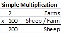
The pivot table has 4 parts to it, which are populated by the fields in your data. A field is a column of data from your original table. Filters, which live at the top of the Pivot Table, filter the data that is summarized below. Rows list all members of a field in rows. Columns list all members of the field in columns. And most importantly Values, are numerical summaries of all the filters rows & columns that have limited your data. The summaries of the values can be changed to do different statistical operations (SUM, AVERAGE, COUNT etc...)

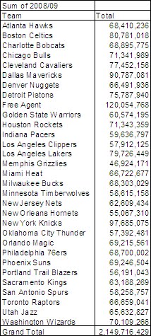
To get our salary by team, we are going to move the 'TEAM' field into the Row area of the pivot table. And the '2008/09' field into the Value part of the pivot table. And voila, you have the following table of salaries spent in 2008/09 by team.

Note that since the data included Free Agents and the salary that the teams who cut them still contractually owe them. The 33 Free Agents in the data add up to the highest paid group of players in 2008/09.

As mentioned SUM is only one of the many summaries a PivotTable can compute. To find our how many players were part of each team, simply right click somewhere in the PivotTables Value section, go to Value Field Settings and in the "Summarize value field by" section select COUNT. You should get the view to the right.

Note, that the Top left area of the Pivot Table automatically includes the summarizing operation and the field it is performing on.

You can find the data and sample PivotTable here so you can play with on your own.

As always, feel free to leave me your questions comments and future blog ideas.

-Danny

Taking & Making Shortcuts in Excel

There are no shortcuts in life, but there are a whole bunch in Excel. And if for some reason it doesn't already exist, you can even make your own.

Excel shortcuts let you quickly maneuver through your window, perform procedures, access user forms or help you preform some excel action with the press of a few keystrokes.

Here is a full list of shortcuts, published by Microsoft. However, if reading through pages of information isn't your thing, here is a shortened list of all the single press shortcuts.

If an Excel shortcut does not already exist for something you do regularly, you can record a macro that does that something and assign a particular code to it.

For example, let's say you have a workbook with multiple worksheets and you always find yourself having to go to a particular sheet (maybe because that is where you keep all your assumptions). You could record a macro that always takes you to the first sheet.

In Excel 2007, you will need to make the "Developer" ribbon available by going into Home > Excel Options > Show Developer Tab in Ribbon. Before you begin recording make sure you are on a different sheet than the one you will want to always switch to. Start the record wizzard:

Give your macro a name ("AssumptionSelect") and enter a shortcut key ("CTRL" + SHIFT + H). [NOTE: be careful not to pick a shortcut that exists because you will overwrite it] Then select whether you want this macro to live ONLY in this workbook or in your instance of excel (so you can always use it, for the specific thing we are recording here you should save it to the workbook only). Click OK to start recording. Select the "Assumption" tab of your workbook and stop recording.

Now whenever you want to go to your assumption tab, just enter your shortcut keys and you are there.


Attached is a workbook that has this macro stored into it.

As always leave me your questions/comments/and future blog ideas.

-Danny

Charts: Visual Evidence

A picture says a thousand words, in Excel we call those pictures charts.

Charts are visual evidence we use to help prove an argument. The difficult part of a chart is "knowing" what you are trying to prove. You could always just start highlighting data and charting it until something looks interesting but starting with an argument makes charting much easier.

Once you know what you want to chart its just a matter of organizing the data in a table, clicking the insert table wizard and adding any additional formats that help prove your message. (Tables may sound intimidating but its just a simple, structured way of organizing data... I will explain more in a future tip)

Example (from GraphJam):

see more Funny Graphs

The message is simple. The chart, even if the data is fictitious, proves the message "Stranger's don't like to get petted"

This is how you would make this chart.

Organize your data into a table that looks like this:

Then you will have to add Titles to the Chart & Axese. The last trick will be to format the Y Axis as a white text color before adding a text box with your custom labels to your charts drawing layer.

Here is a link to the chart recreated in Excel for you to play with.

As always, feel free to leave comments/questions/suggestions.

-Danny